2020-06-19

【R言語と日英翻訳】「reticulate」パッケージを使えば、Pythonライブラリがインポート・実行できる。そして、R上で「googletrans」を用いた日英翻訳をやってみた件

Python - Googletrans R Python テキスト処理翻訳 R - reticulate R - googleLanguageR Homebrew - python

はじめに
googletransライブラリのメリット・デメリット
googletransのインストール
reticulateのセットアップ
RからPython googletransを呼び出す
googletransの実行
まとめ
補足
- Rから、Python ライブラリのヘルプ表示
- googleLanguageRの「No authorization yet in this session!」問題を解決するのは面倒そう！【6/27追加】
参考資料

はじめに

Rの reticulateパッケージは、Python と R の連携性を高めるツール群である*1。

つまりは、Rセッション内でPythonのスクリプトやライブラリをインポートして、シームレスにPythonコードを実行できるなど、RからPythonを呼び出すことができる。

また、RとPythonのオブジェクト間の変換も可能である（Ex. R データフレーム <=> Pandas）。

reticulate::importを使用して、R上で、googletransライブラリを読み込んで、日=>英翻訳、戻し翻訳をやってみる。

`googletransライブラリ`のメリット・デメリット

Googletransは、Google翻訳APIを実装した、無料のPythonライブラリである。

メリット

翻訳速度が早い - translate.google.comと同じサーバー使用
自動言語検出
バルク翻訳
カスタマイズ可能なサービスURL
HTTP/2 サポート

デメリット

１日に使用できる回数制限
テキストは最大15kまで
安定性がいまいち
Googleで正式に提供するAPI Google Cloud Translation は有料

googletransのインストール

まずは、ターミナルを立ち上げて、 pipで、googletransをインストールする。

（2021/6/4に修正）

pip uninstall googletrans

pip install googletrans==4.0.0-rc1

qiita.com

Pythonとpipの設定はこちらの記事を参照のこと。

https://skume.hatenablog.com/entry/2020/05/10/225341skume.hatenablog.com

`reticulate`のセットアップ

Rを起動して、reticulateをインストールして、ロードする。

install.packages("reticulate")
library(reticulate)

Pythonパスを選択して、reticulate::py_config()で確認する。

reticulate::use_python("/usr/local/bin/python", required =T)

reticulate::py_config()

#python:         /usr/local/bin/python
#libpython:      /usr/local/opt/python/Frameworks/Python.framework/Versions/3.7/lib/python3.7/config-3.7m-darwin/libpython3.7.dylib
#pythonhome:     /usr/local/Cellar/python/3.7.7/Frameworks/Python.framework/Versions/3.7:/usr/local/Cellar/python/3.7.7/Frameworks/Python.framework/Versions/3.7
#version:        3.7.7 (default, Mar 10 2020, 15:43:33)  [Clang 11.0.0 (clang-1100.0.33.17)]
#numpy:          /Users/skume/Library/Python/3.7/lib/python/site-packages/numpy
#numpy_version:  1.16.3
#
#NOTE: Python version was forced by use_python function

/usr/local/bin/pythonとなっており、これでOK。

Rから`Python googletrans`を呼び出す

Pythonライブラリのインポートには、 reticulate::import関数を使う。

gt <- reticulate::import(module = "googletrans")

# GtにTranslator関数を渡す
Gt <- gt$Translator()

ヘルプ表示については、補足を参照のこと。

googletransの実行

挨拶の基本として、こんにちわを英訳してみる。

Result <- Gt$translate(text="こんにちわ", src="ja", dest='en')

class(Result)
#[1] "googletrans.models.Translated"
#[2] "python.builtin.object"        

Result
#Translated(src=ja, dest=en, text=Hello, pronunciation=None, extra_data="{'translat...")
#"text="の後ろが、翻訳された結果

translateのオプション

text: 翻訳する文字列

src: 元文の言語(指定無しなら、自動判定)

ja: 日本語, en: 英語, de: ドイツ語, ko: 韓国語, fr: フランス語

dest: 翻訳したい言語(指定無しなら、英語)

結果が"googletrans.models.Translated"で返ってくるので、"text="後の翻訳された結果を抜き出すスクリプトが必要となる。

ここでは、CutTextという関数を新たに定義してみる。

"CutText" <- function(x){
  strsplit(strsplit(as.character(x), ", text=")[[1]][2], ", pronunciation=")[[1]][1]
  }

a <- CutText(Result)
a

#[1] "Hello"

もう少し長い文章で、実行してみる。

例文

Googleの無料サービスなら、単語、フレーズ、ウェブページを英語から100以上の他言語にすぐに翻訳できます。

ResultX <- Gt$translate(text="Googleの無料サービスなら、単語、フレーズ、ウェブページを英語から100以上の他言語にすぐに翻訳できます。", 
                        src="ja", dest='en')

b <- CutText(ResultX)
b

#[1] "With Google's free service, you can instantly translate words, 
#phrases and web pages from English into over 100 other languages."

#さらに、戻し翻訳をしてみると

ResultY <- Gt$translate(text=b, src="en", dest='ja')
c <- CutText(ResultY)
c

#[1] "Googleの無料サービスを利用すると、単語、フレーズ、ウェブページを
#英語から他の100以上の言語に即座に翻訳できます。"

結果、ほぼ違和感なく、戻し翻訳もできている。

まとめ

R上で、日英翻訳ができれば、いちいちGoogle翻訳のページにいかなくても良くなるので、少しだけ便利かも。

最終的には、上記全てを組み込み関数にしたいところ、、

補足

Rから、Python ライブラリのヘルプ表示

#py_help(gt)
#OR
#py_help(gt$client$Translator)
#OR
#py_help(gt$Translator)
#OR
py_help(gt$Translator$translate)

以下が、ヘルプの表示結果

Help on class Translator in module googletrans.client:

class Translator(builtins.object)
 |  Translator(service_urls=None, user_agent='Mozilla/5.0 (Windows NT 10.0; Win64; x64)', raise_exception=False, proxies: Dict[str, httpcore._sync.base.SyncHTTPTransport] = None, timeout: httpx._config.Timeout = None)
 |  
 |  Google Translate ajax API implementation class
 |  
 |      You have to create an instance of Translator to use this API
 |  
 |      :param service_urls: google translate url list. URLs will be used randomly.
 |                           For example ``['translate.google.com', 'translate.google.co.kr']``
 |      :type service_urls: a sequence of strings
 |  
 |      :param user_agent: the User-Agent header to send when making requests.
 |      :type user_agent: :class:`str`
 |  
 |      :param proxies: proxies configuration.
 |                      Dictionary mapping protocol or protocol and host to the URL of the proxy
 |                      For example ``{'http': 'foo.bar:3128', 'http://host.name': 'foo.bar:4012'}``
 |      :type proxies: dictionary
 |  
 |      :param timeout: Definition of timeout for httpx library.
 |                      Will be used for every request.
 |      :type timeout: number or a double of numbers
 |  ||||||| constructed merge base
 |      :param proxies: proxies configuration.
 |                      Dictionary mapping protocol or protocol and host to the URL of the proxy
 |                      For example ``{'http': 'foo.bar:3128', 'http://host.name': 'foo.bar:4012'}``
 |      :param raise_exception: if `True` then raise exception if smth will go wrong
 |      :type raise_exception: boolean
 |  
 |  Methods defined here:
 |  
 |  __init__(self, service_urls=None, user_agent='Mozilla/5.0 (Windows NT 10.0; Win64; x64)', raise_exception=False, proxies: Dict[str, httpcore._sync.base.SyncHTTPTransport] = None, timeout: httpx._config.Timeout = None)
 |      Initialize self.  See help(type(self)) for accurate signature.
 |  
 |  detect(self, text, **kwargs)
 |      Detect language of the input text
 |      
 |      :param text: The source text(s) whose language you want to identify.
 |                   Batch detection is supported via sequence input.
 |      :type text: UTF-8 :class:`str`; :class:`unicode`; string sequence (list, tuple, iterator, generator)
 |      
 |      :rtype: Detected
 |      :rtype: :class:`list` (when a list is passed)
 |      
 |      Basic usage:
 |          >>> from googletrans import Translator
 |          >>> translator = Translator()
 |          >>> translator.detect('이 문장은 한글로 쓰여졌습니다.')
 |          <Detected lang=ko confidence=0.27041003>
 |          >>> translator.detect('この文章は日本語で書かれました。')
 |          <Detected lang=ja confidence=0.64889508>
 |          >>> translator.detect('This sentence is written in English.')
 |          <Detected lang=en confidence=0.22348526>
 |          >>> translator.detect('Tiu frazo estas skribita en Esperanto.')
 |          <Detected lang=eo confidence=0.10538048>
 |      
 |      Advanced usage:
 |          >>> langs = translator.detect(['한국어', '日本語', 'English', 'le français'])
 |          >>> for lang in langs:
 |          ...    print(lang.lang, lang.confidence)
 |          ko 1
 |          ja 0.92929292
 |          en 0.96954316
 |          fr 0.043500196
 |  
 |  translate(self, text, dest='en', src='auto', **kwargs)
 |      Translate text from source language to destination language
 |      
 |      :param text: The source text(s) to be translated. Batch translation is supported via sequence input.
 |      :type text: UTF-8 :class:`str`; :class:`unicode`; string sequence (list, tuple, iterator, generator)
 |      
 |      :param dest: The language to translate the source text into.
 |                   The value should be one of the language codes listed in :const:`googletrans.LANGUAGES`
 |                   or one of the language names listed in :const:`googletrans.LANGCODES`.
 |      :param dest: :class:`str`; :class:`unicode`
 |      
 |      :param src: The language of the source text.
 |                  The value should be one of the language codes listed in :const:`googletrans.LANGUAGES`
 |                  or one of the language names listed in :const:`googletrans.LANGCODES`.
 |                  If a language is not specified,
 |                  the system will attempt to identify the source language automatically.
 |      :param src: :class:`str`; :class:`unicode`
 |      
 |      :rtype: Translated
 |      :rtype: :class:`list` (when a list is passed)
 |      
 |      Basic usage:
 |          >>> from googletrans import Translator
 |          >>> translator = Translator()
 |          >>> translator.translate('안녕하세요.')
 |          <Translated src=ko dest=en text=Good evening. pronunciation=Good evening.>
 |          >>> translator.translate('안녕하세요.', dest='ja')
 |          <Translated src=ko dest=ja text=こんにちは。 pronunciation=Kon'nichiwa.>
 |          >>> translator.translate('veritas lux mea', src='la')
 |          <Translated src=la dest=en text=The truth is my light pronunciation=The truth is my light>
 |      
 |      Advanced usage:
 |          >>> translations = translator.translate(['The quick brown fox', 'jumps over', 'the lazy dog'], dest='ko')
 |          >>> for translation in translations:
 |          ...    print(translation.origin, ' -> ', translation.text)
 |          The quick brown fox  ->  빠른 갈색 여우
 |          jumps over  ->  이상 점프
 |          the lazy dog  ->  게으른 개
 |  
 |  ----------------------------------------------------------------------
 |  Data descriptors defined here:
 |  
 |  __dict__
 |      dictionary for instance variables (if defined)
 |  
 |  __weakref__
 |      list of weak references to the object (if defined)

googleLanguageRの「No authorization yet in this session!」問題を解決するのは面倒そう！【6/27追加】

Google Cloud Translation API

googleLanguageRというGoogle翻訳のAPIがあるのだが、そのまま実行すると、エラーとなる。

install.packages("googleLanguageR")
library(googleLanguageR)

text <- "to administer medicince to animals is frequently a very difficult matter, and yet sometimes it's necessary to do so"

# 英語 => 日本語 への翻訳
gl_translate(text, target = "ja")$translatedText

#2020-06-27 19:44:48 -- Translating text: 115 characters - 
#  ℹ 2020-06-27 19:44:48 > No authorization yet in this session!
#  ℹ 2020-06-27 19:44:48 > No  .httr-oauth  file exists in current working directory.  Do library authentication steps to provide credentials.
#エラー: Invalid token

https://cran.r-project.org/web/packages/googleAuthR/vignettes/google-authentication-types.html Google authentication types for R

github.com

このあたりで、解決策について、いろいろと議論されているが、設定不要のgoogletransを使うので良いのではないかと思う。

参考資料

pypi.org

rstudio.github.io

*1:https://rstudio.github.io/reticulate/#importing-python-modules

2020-06-18

R/Keras/TensorFlowでやる『ディープラーニング(Deep Learning)』のすゝめ【その１】教師なしニューラルネットワークDeep Autoencoder のsimple modelをやってみた件

R R - Keras R - TensorFlow Deep Learning DL - Autoencoder グラフ可視化人工知能

はじめに
Keras/TensorFlowのセットアップ
手書き文字MNISTデータセットの用意
Autoencoderのモデル構築
まとめ
R/Kerasを用いたDeep Learningの推薦図書
全コード in Gist
補足
- 参考文献

はじめに

Rで、ディープラーニング( Deep Learning )をやるというのが最近の活動である。

【１】では、教師なしニューラルネットワークであるAutoencoder（オートエンコーダー）のsimple modelを実装してみる。

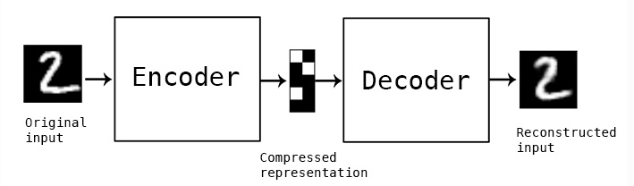
Autoencoder は、Encoder（元データから低次元への変換層）とDecoder（低次元から元データに戻す変換層）からなるニューラルネットワークの特殊系の１つである。 Autoencoderでは、出力層で与える教師データを入力層としても与えることで、入力層と出力層のユニットが同じとなる構造を持つ。

Autoencoderの開発は1980年代に遡り、Hinton と PDPグループが、「教師なしの逆伝播」の問題に対処するために、教師データを入力データとして使用したことに始まる*1 *2。

また、2006年、Hinton と Salakhutdinov は、多層のニューラルネットワークを持つDeep Autoencoderを用いた、手書きアラビア数字画像などの次元圧縮の結果を報告した*3。

彼らは、小さな中央層を持つ多層ニューラルネットワークをトレーニングさせて、高次元の入力ベクトルを出力層で再構築することで、画像データを低次元のコードとして変換できることを示した。また、データの次元数を削減するツールとして、主成分分析よりも、Deep autoencoderのほうが優れていると述べている。

このとき、両者とも画像をいったんベクトルデータに変換しているが、確かに、PCA（下図の左）よりもだいぶ良く見える結果である。

*4の論文より引用

実際に、２次元上に数字画像をプロットした結果がサプリメント図にのっている。

*5のサプリメントデータより引用

今回、R言語のKeras/TensorFlowパッケージを使って、Autoencoderのmodelをいろいろと実装していく。そして、サプリ図のような、数字画像のプロット結果を得ることをゴールにしている。

Rでの、Keras/TensorFlowのインストールについては以下を参照のこと。

keras.rstudio.com

200612_BioPackathon_ss from Satoshi Kume

www.slideshare.net

Keras/TensorFlowのセットアップ

今回、CNN（Convolutional Neural Network: 畳み込みニューラルネットワーク）は使わないので、AutoencoderはCPU実行した。

# Kerasパッケージのロード
library(keras)

# "/usr/local/bin/python"の選択
reticulate::use_python("/usr/local/bin/python", required =T)

ここで、「install_keras()」は特にやらなくても動くはずである。

BrewでインストールしたPythonを使っていて、Pythonのパスは以下のように「/usr/local/bin/python」になっている。

reticulate::py_config()

python:         /usr/local/bin/python
libpython:      /usr/local/opt/python/Frameworks/Python.framework/Versions/3.7/lib/python3.7/config-3.7m-darwin/libpython3.7.dylib
pythonhome:     /usr/local/Cellar/python/3.7.7/Frameworks/Python.framework/Versions/3.7:/usr/local/Cellar/python/3.7.7/Frameworks/Python.framework/Versions/3.7
version:        3.7.7 (default, Mar 10 2020, 15:43:33)  [Clang 11.0.0 (clang-1100.0.33.17)]
numpy:          /Users/skume/Library/Python/3.7/lib/python/site-packages/numpy
numpy_version:  1.16.3
tensorflow:     /usr/local/lib/python3.7/site-packages/tensorflow

NOTE: Python version was forced by use_python function

このあたりの設定についは、過去のブログ記事を参照のこと。

https://skume.hatenablog.com/entry/2020/05/10/225341skume.hatenablog.com

手書き文字MNISTデータセットの用意

Autoencoderは、以下の図のように、中央に圧縮特徴層を持ち、その前後にエンコード層とデコード層の組み合わせとして表される*6。

まずは、あの有名な手書き文字のデータセットをダウンロードしてアレイ型に変換する。

#MNISTのダウンロード
Data <- dataset_mnist()
str(Data)

#アレイ型に変換
xtrain <- Data$train$x
xtrain <- xtrain/255
ytrain <- Data$train$y

xtest <- Data$test$x
xtest <- xtest/255
ytest <- Data$test$y

今回、2D画像は一次元ベクトルに変換して入力データとするため inputユニットサイズ = ピクセル数となり、それを計算しておく。

# インプットデータサイズの計算
dim(xtrain)

input_size <- dim(xtrain)[2]*dim(xtrain)[3]

input_size

inputサイズは、28 x 28 = 784ユニットとなる。

さらに、３次元アレイ（1: 画像、2: X、3: Y）から、２次元アレイ（1: 画像、2: 一次元ベクトル）に変換する。

dim(xtrain)
#[1] 60000    28    28
dim(xtest)
#[1] 10000    28    28

#２次元アレイに変換
x_train = array_reshape(xtrain, dim=c(dim(xtrain)[1], input_size))
x_test = array_reshape(xtest, dim=c(dim(xtest)[1], input_size))

dim(x_train)
#[1] 60000   784
dim(x_test)
#[1] 10000   784

Autoencoderのモデル構築

ここから、実際のAutoencoderのモデル構築を行う。

Rでは、パイプ文法（%>%）でモデルを書いていく。

シンプルAutoencoderモデル０１

input1 <- layer_input(shape = input_size)
output1 <- input1 %>% 
  layer_dense(units=256, activation = "relu") %>% 
  layer_activation_leaky_relu() %>% 
  layer_dense(units=2) %>% 
  layer_activation_leaky_relu() %>%
  layer_dense(units=256, activation = "relu") %>% 
  layer_activation_leaky_relu() %>% 
  layer_dense(units = input_size, activation = "sigmoid") %>% 
  layer_activation_leaky_relu()

# モデル構築
Autoencoder1 <- keras_model(input1, output1)

モデルをsummaryで表示してみる。

summary(Autoencoder1)

#Model: "model"
#___________________________________________________________
#Layer (type)              Output Shape            Param #  
#===========================================================
#input_1 (InputLayer)      [(None, 784)]           0        
#___________________________________________________________
#dense (Dense)             (None, 256)             200960   
#___________________________________________________________
#leaky_re_lu (LeakyReLU)   (None, 256)             0        
#___________________________________________________________
#dense_1 (Dense)           (None, 2)               514      
#___________________________________________________________
#leaky_re_lu_1 (LeakyReLU) (None, 2)               0        
#___________________________________________________________
#dense_2 (Dense)           (None, 256)             768      
#___________________________________________________________
#leaky_re_lu_2 (LeakyReLU) (None, 256)             0        
#___________________________________________________________
#dense_3 (Dense)           (None, 784)             201488   
#___________________________________________________________
#leaky_re_lu_3 (LeakyReLU) (None, 784)             0        
#===========================================================
#Total params: 403,730
#Trainable params: 403,730
#Non-trainable params: 0
#___________________________________________________________

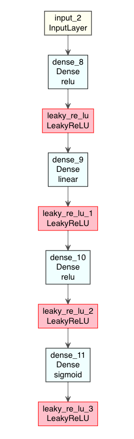
DLのモデルはグラフ構造の方が見やすいので、モデルの図示を試してみる。

Rでは、deepvizパッケージ*7で、ニューラルネットワーク構造を可視化できる。

ただ、deepvizは色合いが短調なので、ここでは改変版のplot_model_modiで行う。

# Gistで公開している plot_model_modi のロード
source("https://gist.githubusercontent.com/kumeS/41fed511efb45bd55d468d4968b0f157/raw/07da3ba4a2e477f352d03e8b5ac00d394fe9afec/DL_plot_modi_v1.1.R")

#Autoencoder1モデルの図示
modelplot <- Autoencoder1
modelplot %>% plot_model_modi()

（plot_model_modiの出力結果）

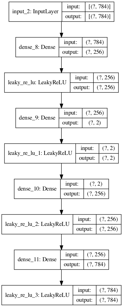
また、Python TensorFlowでのplot_modelを行いたい場合には、 R上に、PythonのTensorFlowパッケージをロードすれば、グラフ出力ができる。

#Python Tensorflowのplot_modelを使う

tf <- reticulate::import(module = "tensorflow")
py_plot_model <- tf$keras$utils$plot_model
py_plot_model(modelplot, to_file='model1.png', 
              show_shapes=T, show_layer_names=T, 
              expand_nested=T, dpi=100)

（Python Tensorflowのplot_modelの出力結果）

次に、モデルのコンパイルを行う。最適化アルゴリズムはrmspropのデフォルト値、損失関数はmean_squared_errorにしている。

# Compile
Autoencoder1 %>% compile(optimizer="rmsprop", loss="mean_squared_error")

そして、フィットでAutoencoderを実行する。

# Fit
Autoencoder1 %>% fit(x_train, x_train, epochs=100, batch_size=1000)

次に、AutoencoderによるTrainデータセットの変換結果を確認する。

まずは、アレイ型を２次元から3次元に変換する。

pred_imgs1 <- Autoencoder1 %>% predict(x_train)
pred_imgsR1 <- array_reshape(pred_imgs1, dim=c(dim(pred_imgs1)[1], 28, 28))

dim(pred_imgsR1)
#[1] 60000    28    28

#Testデータセットについて
#（今回はスキップ）
#pred_imgsY1 = Autoencoder %>% predict(x_test)
#pred_imgsRY1 = array_reshape(pred_imgsY1, dim=c(dim(pred_imgsY1)[1], 28, 28))

手書き文字を表示するのに、まずは、 BioconductorのEBImage*8をインストールする。

if (!requireNamespace("BiocManager", quietly = TRUE)){install.packages("BiocManager")}
BiocManager::install("EBImage")

#EBImageをロードする
library(EBImage)

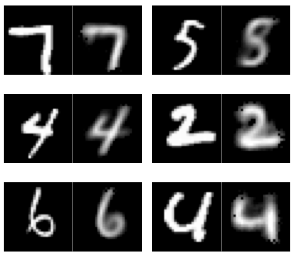
input画像とAutoencoderをかけた後の画像の結果を並べて表示してみる。

par(mfrow=c(3,2))
for (i in 1:6) {
m <- sample(1:dim(xtrain)[1], 1, replace = F)
display(combine(t(xtrain[m,,]), t(pred_imgsR1[m,,])), 
        method="raster", nx=2, all=TRUE, spacing = 0.01, margin = 2)
}

入力（左側）と出力（右側）の結果を示す。

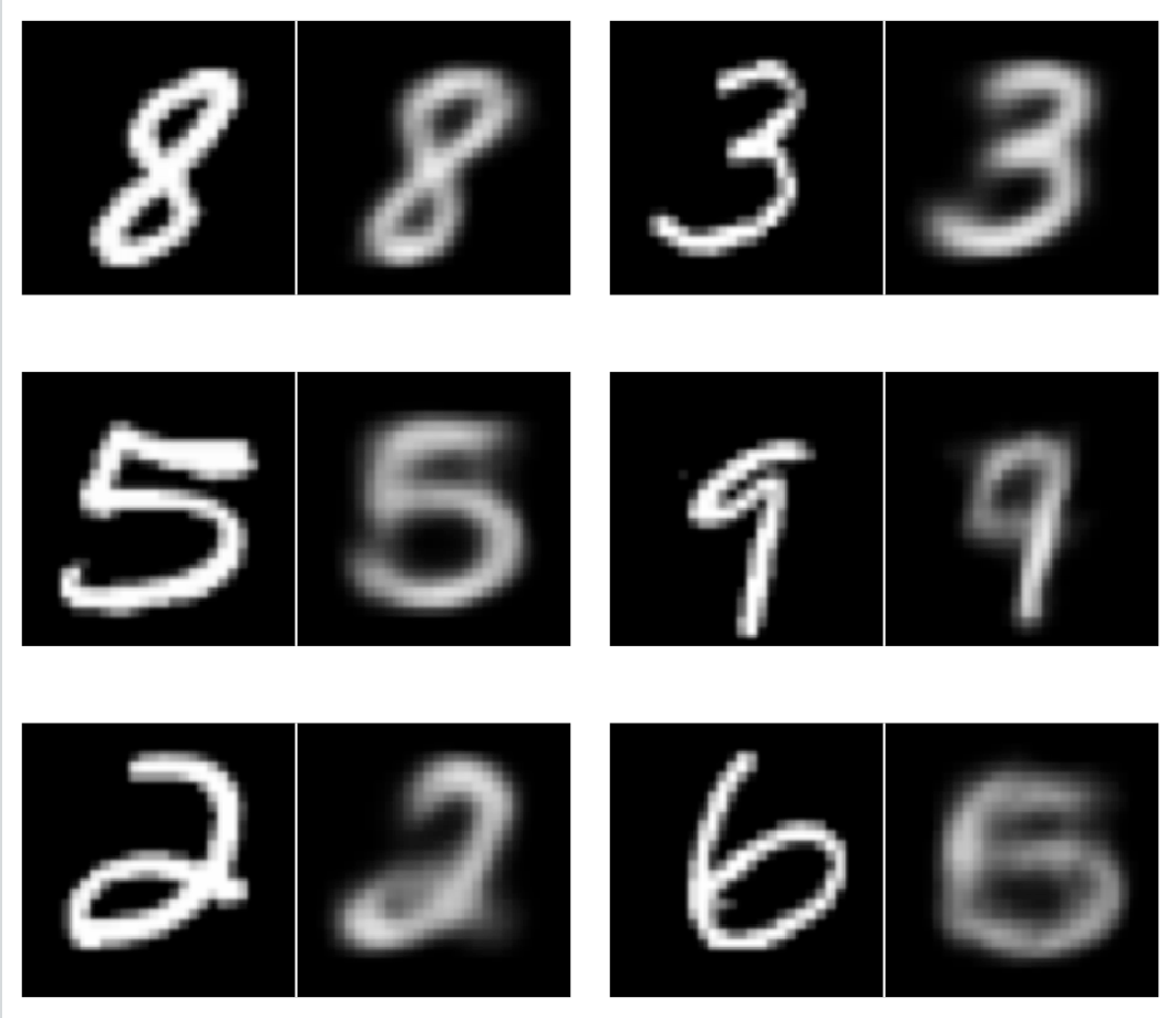
やはり論文のサプリ図のように、圧縮特徴層を取り出して、文字画像データを図上にプロットしたくなる。

まずは、中間層を抜き出して、２次元プロットを試みる。

#Autoencoderの中間層までのモデルを抜き出す
intermediate_layer <- keras_model(inputs = Autoencoder1$input,
                                        outputs = get_layer(Autoencoder1, "dense_1")$output)

summary(intermediate_layer)
#Model: "model_1"
#____________________________________________________________________
#Layer (type)                  Output Shape               Param #    
#====================================================================
#input_1 (InputLayer)          [(None, 784)]              0          
#____________________________________________________________________
#dense (Dense)                 (None, 256)                200960     
#____________________________________________________________________
#leaky_re_lu (LeakyReLU)       (None, 256)                0          
#____________________________________________________________________
#dense_1 (Dense)               (None, 2)                  514        
#====================================================================
#Total params: 201,474
#Trainable params: 201,474
#Non-trainable params: 0
#____________________________________________________________________

#さらに、中間層まで変換をpredictする
intermediate_output <- predict(intermediate_layer, x_train)

とりあえず、色付きマーカーで2Dプロットをしてみる。

全てのデータ（6万点）だと多過ぎるので、５００点分をランダムサンプリングして表示した。

xy <- data.frame(ytrain, intermediate_output)
Sam <- sample(1:nrow(xy), 500, replace = F)
xy1 <- xy[Sam,]
par(mfrow=c(1,1), mai=c(0.75,0.75,0.2,0.2), mgp = c(2.5,1,0))
plot(xy1[,2:3], pch=21, cex=0.75, bg=rainbow(10)[xy1[,1]+1])

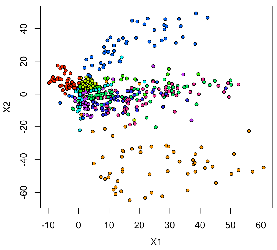
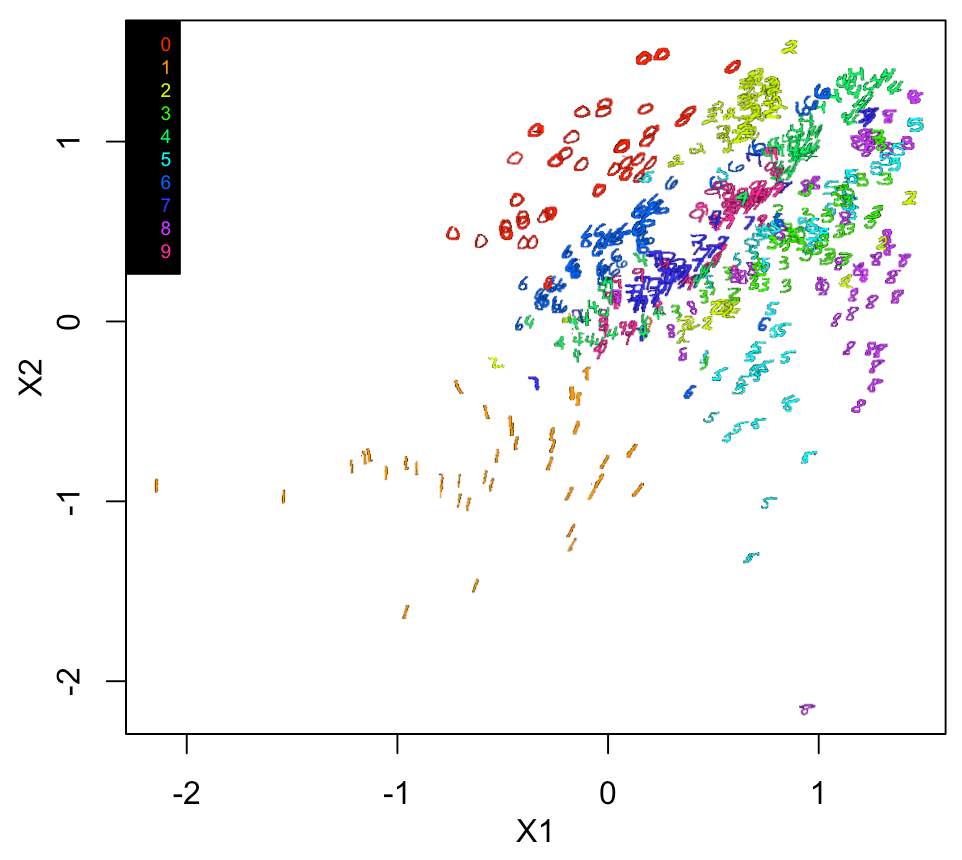
やはり、実際の数字画像でプロットしないと雰囲気が出ない。

ちょっと面倒なのだが、空白のプロットをして、そこにラスター画像を重ねていくとできる。ラスター画像は背景を透明にしているのがひと工夫である。

#まずは、空白のプロットをしてみる
plot(xy1[,2:3], pch=21, cex=0.1, col="white")

##そこに、画像を色付きでプロットする
for(n in 1:nrow(xy1)){
  #n <-4
  v <- col2rgb(rainbow(10)[xy1[n,1] + 1]) / 255
  img = channel(xy2[n,,], 'rgb')
  img[,,1] <- img[,,1]*v[1]
  img[,,2] <- img[,,2]*v[2]
  img[,,3] <- img[,,3]*v[3]
  ff <- t(as.raster(img))
  ff[ff == "#000000"] <- "#00000000"
  rasterImage(ff, xy1[n,2]-1.5, xy1[n,3]-1.5, 
              xy1[n,2]+1.5, xy1[n,3]+1.5)
}

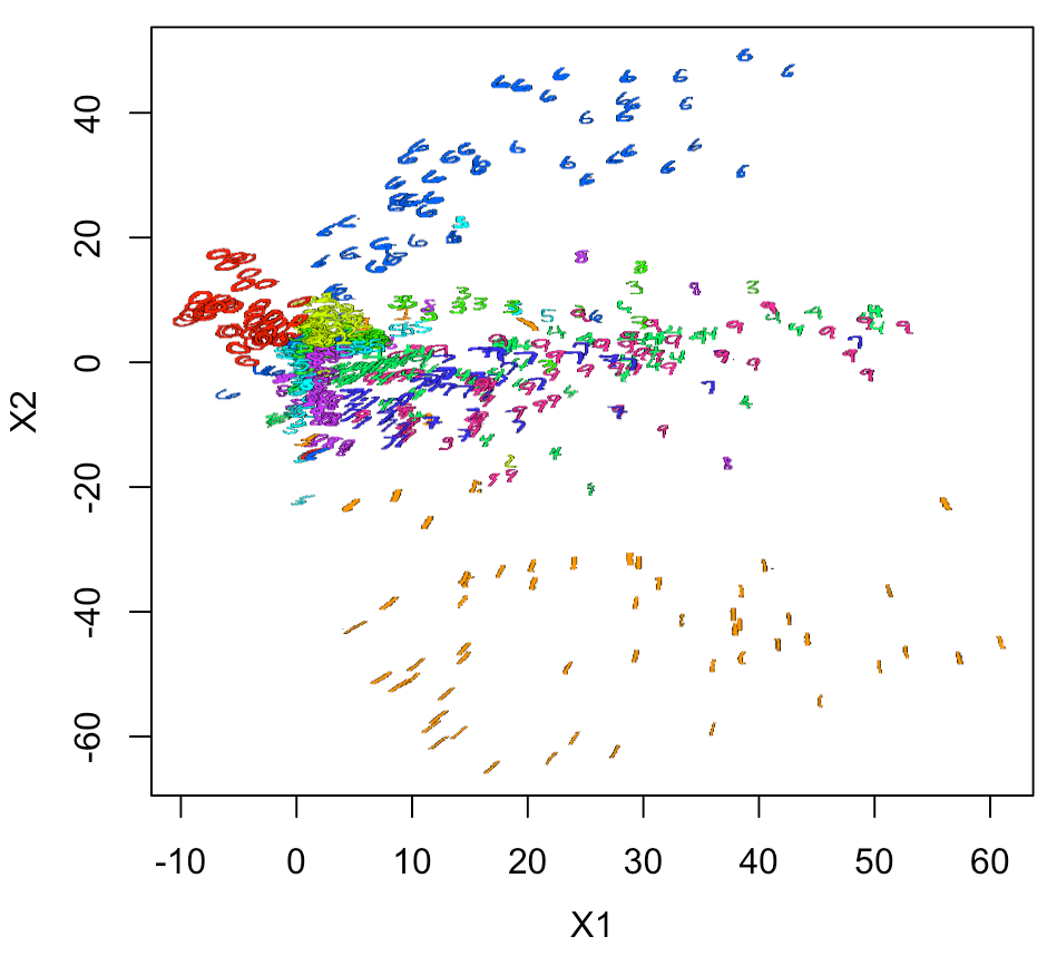
プロット結果として考察できることは、このモデルは、０、１、６以外ではあまり精度が良くない。

そこで、別モデルもいくつか試してみる。

RStudioセッションの初期化

レイヤーが連番となるため、DL実行ごとに、いったん、Rセッションを初期化しておくのが無難・・・

.rs.restartR()

library(keras)

library(EBImage)

reticulate::use_python("/usr/local/bin/python", required =T)

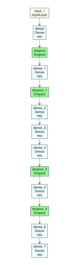
シンプルAutoencoderモデル０２

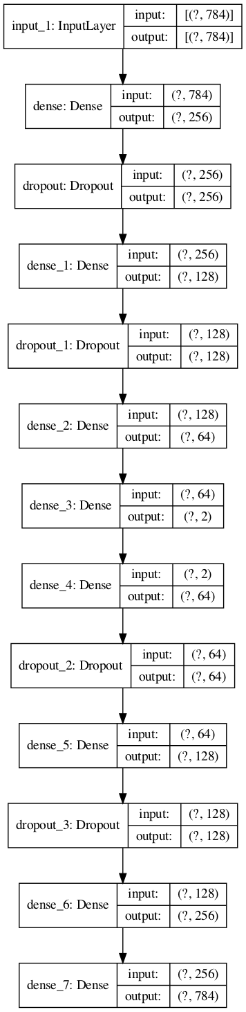
このモデルでは、少しレイヤー数を増やして、Dropoutも入れてみた。活性化関数は、reluにしている。

input2 <- layer_input(shape = input_size) 
output2 <- input2 %>% 
  layer_dense(units = 256, activation = "relu") %>% 
  layer_dropout(rate = 0.2) %>% 
  layer_dense(units = 128, activation = "relu") %>%
  layer_dropout(rate = 0.1) %>%
  layer_dense(units = 64, activation = "relu") %>%
  layer_dense(units = 2, activation = "relu") %>%
  layer_dense(units = 64, activation = "relu") %>% 
  layer_dropout(rate = 0.1) %>% 
  layer_dense(units = 128, activation = "relu") %>%
  layer_dropout(rate = 0.2) %>%
  layer_dense(units = 256, activation = "relu") %>%
  layer_dense(units = input_size, activation = "relu") 

Autoencoder2 <- keras_model(input2, output2)
summary(Autoencoder2)

モデルをプロットするとこんな感じである。

modelplot <- Autoencoder2
modelplot %>% plot_model_modi()

（plot_model_modiの出力結果）

tf <- reticulate::import(module = "tensorflow")
py_plot_model <- tf$keras$utils$plot_model
py_plot_model(modelplot, to_file='model.png', 
              show_shapes=T, show_layer_names=T, 
              expand_nested=T, dpi=100)

（Python Tensorflowのplot_modelの出力結果）

次に、コンパイル・フィットを実行する。

最適化アルゴリズムはrmspropのデフォルト値、損失関数はmean_squared_errorにしている。

#compile
Autoencoder2 %>% 
  compile(optimizer="rmsprop", loss="mean_squared_error")

#Fit
Autoencoder2 %>% 
  fit(x_train, x_train, epochs=100, batch_size=1000, shuffle=TRUE)

（計算結果）

AutoencoderによるTrainデータセットの変換結果を確認してみると、

pred_imgs2 <- Autoencoder2 %>% predict(x_train)
pred_imgsR2 <- array_reshape(pred_imgs2, dim=c(dim(pred_imgs2)[1], 28, 28))
dim(pred_imgsR2)

par(mfrow=c(3,2))
for (i in 1:6) {
  m <- sample(1:dim(xtrain)[1], 1, replace = F)
  display(combine(t(xtrain[m,,]), t(pred_imgsR2[m,,])), 
          method="raster", nx=2, all=TRUE, spacing = 0.01, margin = 2)
}

入力（左側）と出力（右側）の結果を示す。

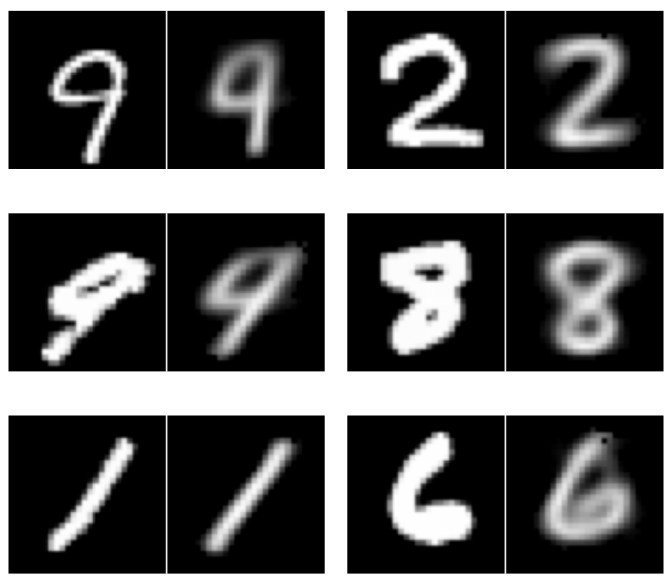
同じく、中間層の圧縮特徴量でプロットしてみる。

##中間層の取得
summary(Autoencoder2)
intermediate_layer <- keras_model(inputs = Autoencoder2$input,
                                  outputs = get_layer(Autoencoder2, "dense_3")$output)
summary(intermediate_layer)
intermediate_output <- predict(intermediate_layer, x_train)

#2Dプロット
xy <- data.frame(ytrain, intermediate_output)
Sam <- sample(1:nrow(xy), 500, replace = F)
xy1 <- xy[Sam,]
par(mfrow=c(1,1), mai=c(0.75,0.75,0.2,0.2), mgp = c(2.5,1,0))
plot(xy1[,2:3], pch=21, cex=0.75, bg=rainbow(10)[xy1[,1]+1])

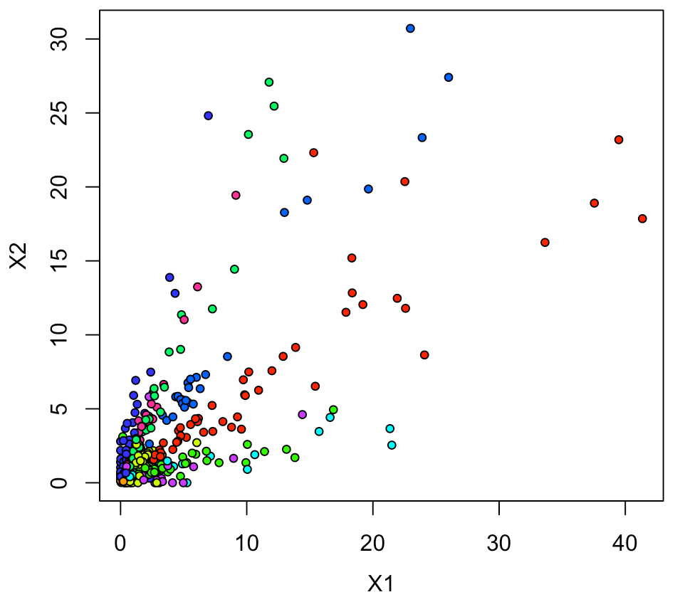
これでは、データ点がゼロ付近に密集している印象なので、 XY軸それぞれでlog10をとることで、それが解消できるか試してみる。

そうすると、結構いい感じでプロットされた。

xy1[,2:3] <- log10(xy1[,2:3])

plot(xy1[,2:3], pch=21, cex=0.75, bg=rainbow(10)[xy1[,1]+1])

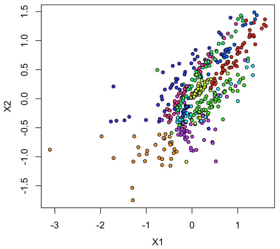
次に、Log10をとったXY座標で、実際の画像での2Dプロットをやってみると

xy2 <- xtrain[Sam,,]

#空白のプロット
plot(xy1[,2:3], pch=21, cex=0.1, col="white")

##プロット全体のXY座標サイズを考慮して、全体の3%の大きさでプロットする
a <- range(xy1[,2][is.finite(xy1[,2])])
b <- range(xy1[,3][is.finite(xy1[,3])])
a1 <- diff(a)*0.015
b1 <- diff(b)*0.015

##色付き画像でプロットする
for(n in 1:nrow(xy1)){
  #n <-4
  v <- col2rgb(rainbow(10)[xy1[n,1] + 1]) / 255
  img = channel(xy2[n,,], 'rgb')
  img[,,1] <- img[,,1]*v[1]
  img[,,2] <- img[,,2]*v[2]
  img[,,3] <- img[,,3]*v[3]
  ff <- t(as.raster(img))
  ff[ff == "#000000"] <- "#00000000"
  rasterImage(ff, xy1[n,2]-a1, xy1[n,3]-b1, 
              xy1[n,2]+a1, xy1[n,3]+b1)
}

結構良い感じにできる。

シンプルAutoencoderモデル０３

最後に、論文あった、レイヤーのユニット数（784-1000-500-250-2）で実装してみる。

３回目なので、説明はやや端折り気味で。。

input3 <- layer_input(shape = input_size) 
output3 <- input3 %>% 
  layer_dense(units = 1000, activation = "relu") %>% 
  layer_dense(units = 500, activation = "relu") %>%
  layer_dense(units = 250, activation = "relu") %>%
  layer_dense(units = 2, activation = "relu") %>%
  layer_dense(units = 250, activation = "relu") %>% 
  layer_dense(units = 500, activation = "relu") %>%
  layer_dense(units = 100, activation = "relu") %>%
  layer_dense(units = input_size, activation = "relu") 

Autoencoder3 <- keras_model(input3, output3)

summary(Autoencoder3)

#Model: "model"
#______________________________________________________________________
#Layer (type)                   Output Shape                Param #    
#======================================================================
#input_1 (InputLayer)           [(None, 784)]               0          
#______________________________________________________________________
#dense (Dense)                  (None, 1000)                785000     
#______________________________________________________________________
#dense_1 (Dense)                (None, 500)                 500500     
#______________________________________________________________________
#dense_2 (Dense)                (None, 250)                 125250     
#______________________________________________________________________
#dense_3 (Dense)                (None, 2)                   502        
#______________________________________________________________________
#dense_4 (Dense)                (None, 250)                 750        
#______________________________________________________________________
#dense_5 (Dense)                (None, 500)                 125500     
#______________________________________________________________________
#dense_6 (Dense)                (None, 100)                 50100      
#______________________________________________________________________
#dense_7 (Dense)                (None, 784)                 79184      
#======================================================================
#Total params: 1,666,786
#Trainable params: 1,666,786
#Non-trainable params: 0
#______________________________________________________________________

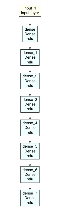
モデルを図示すると、

modelplot <- Autoencoder3
modelplot %>% plot_model_modi(width=1, height=1.25)

（plot_model_modiの出力結果）

続けて、コンパイルして、フィットを実行する。

#compile
Autoencoder3 %>%
  compile(optimizer="rmsprop", loss="mean_squared_error")

#Fit
Autoencoder3 %>% 
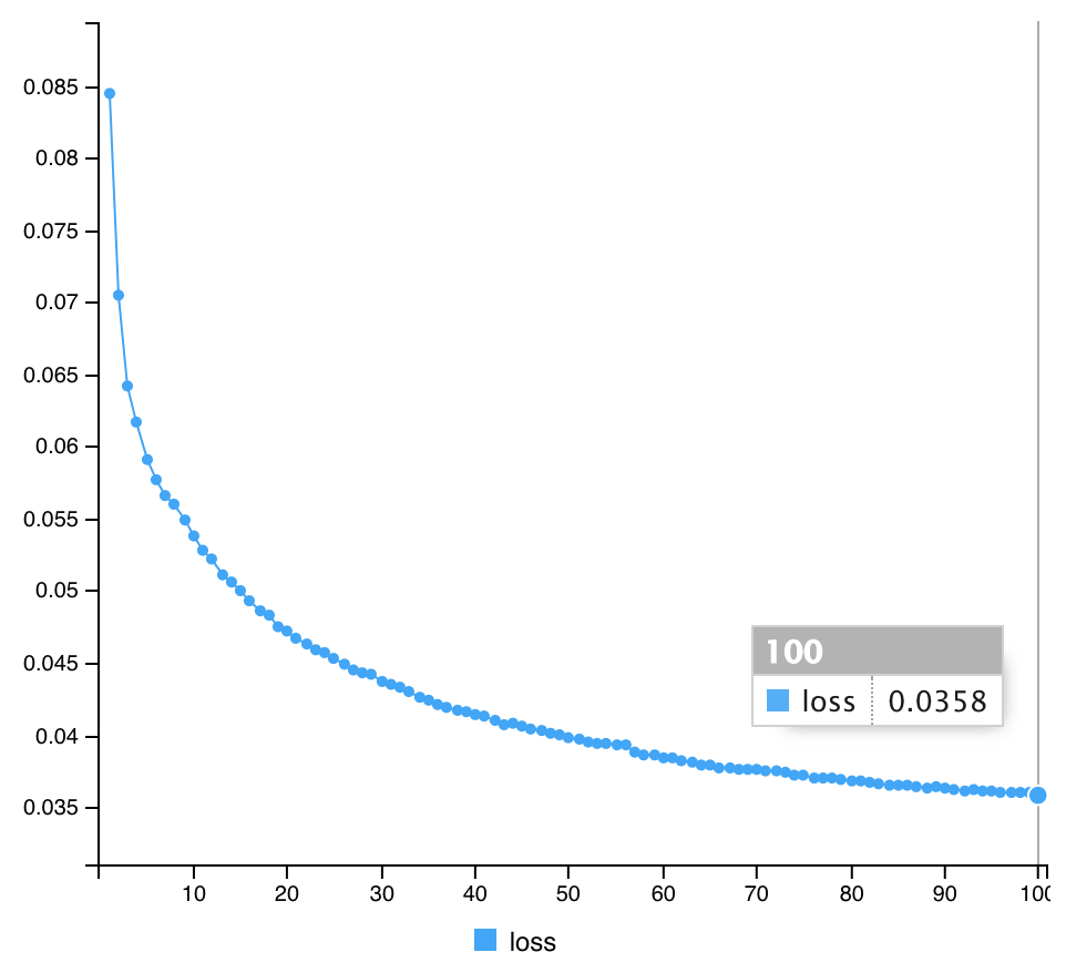
  fit(x_train, x_train, epochs=100, batch_size=1000, shuffle=TRUE)

#計算途中の出力
Epoch 1/100
60/60 [==============================] - 3s 48ms/step - loss: 0.0845
Epoch 2/100
60/60 [==============================] - 3s 43ms/step - loss: 0.0705
Epoch 3/100
60/60 [==============================] - 3s 43ms/step - loss: 0.0642
Epoch 4/100
60/60 [==============================] - 3s 52ms/step - loss: 0.0617
Epoch 5/100
60/60 [==============================] - 3s 46ms/step - loss: 0.0591
Epoch 6/100
60/60 [==============================] - 3s 44ms/step - loss: 0.0577
Epoch 7/100
60/60 [==============================] - 3s 42ms/step - loss: 0.0566
Epoch 8/100
60/60 [==============================] - 2s 42ms/step - loss: 0.0560
Epoch 9/100
60/60 [==============================] - 3s 42ms/step - loss: 0.0549
Epoch 10/100
60/60 [==============================] - 3s 47ms/step - loss: 0.0538
Epoch 11/100
60/60 [==============================] - 3s 47ms/step - loss: 0.0528
Epoch 12/100
60/60 [==============================] - 3s 47ms/step - loss: 0.0522
Epoch 13/100
60/60 [==============================] - 3s 46ms/step - loss: 0.0511
Epoch 14/100
60/60 [==============================] - 3s 44ms/step - loss: 0.0506
Epoch 15/100
60/60 [==============================] - 3s 42ms/step - loss: 0.0500
Epoch 16/100
60/60 [==============================] - 3s 43ms/step - loss: 0.0493
Epoch 17/100
60/60 [==============================] - 3s 43ms/step - loss: 0.0486
Epoch 18/100
60/60 [==============================] - 3s 43ms/step - loss: 0.0483
Epoch 19/100
60/60 [==============================] - 3s 43ms/step - loss: 0.0475
Epoch 20/100
60/60 [==============================] - 3s 43ms/step - loss: 0.0472
Epoch 21/100
60/60 [==============================] - 3s 43ms/step - loss: 0.0467
Epoch 22/100
60/60 [==============================] - 3s 42ms/step - loss: 0.0463
Epoch 23/100
60/60 [==============================] - 3s 42ms/step - loss: 0.0459
Epoch 24/100
60/60 [==============================] - 3s 43ms/step - loss: 0.0457
Epoch 25/100
60/60 [==============================] - 3s 44ms/step - loss: 0.0453
Epoch 26/100
60/60 [==============================] - 3s 42ms/step - loss: 0.0449
Epoch 27/100
60/60 [==============================] - 3s 43ms/step - loss: 0.0445
Epoch 28/100
60/60 [==============================] - 3s 43ms/step - loss: 0.0443
Epoch 29/100
60/60 [==============================] - 3s 45ms/step - loss: 0.0442
Epoch 30/100
60/60 [==============================] - 3s 44ms/step - loss: 0.0437
Epoch 31/100
60/60 [==============================] - 3s 49ms/step - loss: 0.0435
Epoch 32/100
60/60 [==============================] - 4s 62ms/step - loss: 0.0433
Epoch 33/100
60/60 [==============================] - 5s 79ms/step - loss: 0.0430
Epoch 34/100
60/60 [==============================] - 4s 65ms/step - loss: 0.0426
Epoch 35/100
60/60 [==============================] - 3s 48ms/step - loss: 0.0424
Epoch 36/100
60/60 [==============================] - 3s 43ms/step - loss: 0.0421
Epoch 37/100
60/60 [==============================] - 3s 42ms/step - loss: 0.0419
Epoch 38/100
60/60 [==============================] - 3s 45ms/step - loss: 0.0417
Epoch 39/100
60/60 [==============================] - 3s 44ms/step - loss: 0.0416
Epoch 40/100
60/60 [==============================] - 3s 45ms/step - loss: 0.0414
Epoch 41/100
60/60 [==============================] - 3s 47ms/step - loss: 0.0413
Epoch 42/100
60/60 [==============================] - 3s 46ms/step - loss: 0.0410
Epoch 43/100
60/60 [==============================] - 3s 46ms/step - loss: 0.0407
Epoch 44/100
60/60 [==============================] - 3s 47ms/step - loss: 0.0408
Epoch 45/100
60/60 [==============================] - 3s 43ms/step - loss: 0.0406
Epoch 46/100
60/60 [==============================] - 3s 43ms/step - loss: 0.0404
Epoch 47/100
60/60 [==============================] - 3s 44ms/step - loss: 0.0403
Epoch 48/100
60/60 [==============================] - 3s 46ms/step - loss: 0.0401
Epoch 49/100
60/60 [==============================] - 3s 43ms/step - loss: 0.0400
Epoch 50/100
60/60 [==============================] - 3s 43ms/step - loss: 0.0398
Epoch 51/100
60/60 [==============================] - 3s 43ms/step - loss: 0.0397
Epoch 52/100
60/60 [==============================] - 3s 42ms/step - loss: 0.0395
Epoch 53/100
60/60 [==============================] - 3s 43ms/step - loss: 0.0394
Epoch 54/100
60/60 [==============================] - 3s 45ms/step - loss: 0.0394
Epoch 55/100
60/60 [==============================] - 3s 48ms/step - loss: 0.0393
Epoch 56/100
60/60 [==============================] - 3s 45ms/step - loss: 0.0393
Epoch 57/100
60/60 [==============================] - 3s 45ms/step - loss: 0.0388
Epoch 58/100
60/60 [==============================] - 3s 43ms/step - loss: 0.0386
Epoch 59/100
60/60 [==============================] - 3s 42ms/step - loss: 0.0386
Epoch 60/100
60/60 [==============================] - 3s 50ms/step - loss: 0.0384
Epoch 61/100
60/60 [==============================] - 3s 45ms/step - loss: 0.0384
Epoch 62/100
60/60 [==============================] - 3s 46ms/step - loss: 0.0382
Epoch 63/100
60/60 [==============================] - 3s 52ms/step - loss: 0.0381
Epoch 64/100
60/60 [==============================] - 3s 50ms/step - loss: 0.0379
Epoch 65/100
60/60 [==============================] - 3s 46ms/step - loss: 0.0379
Epoch 66/100
60/60 [==============================] - 3s 47ms/step - loss: 0.0377
Epoch 67/100
60/60 [==============================] - 3s 49ms/step - loss: 0.0377
Epoch 68/100
60/60 [==============================] - 3s 48ms/step - loss: 0.0376
Epoch 69/100
60/60 [==============================] - 3s 49ms/step - loss: 0.0376
Epoch 70/100
60/60 [==============================] - 3s 53ms/step - loss: 0.0376
Epoch 71/100
60/60 [==============================] - 3s 46ms/step - loss: 0.0375
Epoch 72/100
60/60 [==============================] - 3s 44ms/step - loss: 0.0375
Epoch 73/100
60/60 [==============================] - 3s 48ms/step - loss: 0.0374
Epoch 74/100
60/60 [==============================] - 3s 45ms/step - loss: 0.0372
Epoch 75/100
60/60 [==============================] - 3s 43ms/step - loss: 0.0372
Epoch 76/100
60/60 [==============================] - 3s 43ms/step - loss: 0.0370
Epoch 77/100
60/60 [==============================] - 3s 45ms/step - loss: 0.0370
Epoch 78/100
60/60 [==============================] - 3s 43ms/step - loss: 0.0370
Epoch 79/100
60/60 [==============================] - 3s 42ms/step - loss: 0.0369
Epoch 80/100
60/60 [==============================] - 3s 44ms/step - loss: 0.0368
Epoch 81/100
60/60 [==============================] - 3s 52ms/step - loss: 0.0368
Epoch 82/100
60/60 [==============================] - 3s 49ms/step - loss: 0.0367
Epoch 83/100
60/60 [==============================] - 3s 54ms/step - loss: 0.0366
Epoch 84/100
60/60 [==============================] - 3s 44ms/step - loss: 0.0365
Epoch 85/100
60/60 [==============================] - 3s 43ms/step - loss: 0.0365
Epoch 86/100
60/60 [==============================] - 3s 43ms/step - loss: 0.0365
Epoch 87/100
60/60 [==============================] - 3s 43ms/step - loss: 0.0364
Epoch 88/100
60/60 [==============================] - 3s 42ms/step - loss: 0.0363
Epoch 89/100
60/60 [==============================] - 3s 42ms/step - loss: 0.0364
Epoch 90/100
60/60 [==============================] - 3s 43ms/step - loss: 0.0363
Epoch 91/100
60/60 [==============================] - 3s 44ms/step - loss: 0.0362
Epoch 92/100
60/60 [==============================] - 3s 44ms/step - loss: 0.0361
Epoch 93/100
60/60 [==============================] - 3s 44ms/step - loss: 0.0362
Epoch 94/100
60/60 [==============================] - 3s 43ms/step - loss: 0.0361
Epoch 95/100
60/60 [==============================] - 3s 42ms/step - loss: 0.0361
Epoch 96/100
60/60 [==============================] - 3s 42ms/step - loss: 0.0360
Epoch 97/100
60/60 [==============================] - 3s 42ms/step - loss: 0.0360
Epoch 98/100
60/60 [==============================] - 3s 42ms/step - loss: 0.0360
Epoch 99/100
60/60 [==============================] - 2s 42ms/step - loss: 0.0360
Epoch 100/100
60/60 [==============================] - 3s 43ms/step - loss: 0.0358

同じく、入力（左側）と出力（右側）の結果を確認する。

pred_imgs3 <- Autoencoder3 %>% predict(x_train)
pred_imgsR3 <- array_reshape(pred_imgs3, dim=c(dim(pred_imgs3)[1], 28, 28))
dim(pred_imgsR3)

par(mfrow=c(3,2))
for (i in 1:6) {
  m <- sample(1:dim(xtrain)[1], 1, replace = F)
  display(combine(t(xtrain[m,,]), t(pred_imgsR3[m,,])), 
          method="raster", nx=2, all=TRUE, spacing = 0.01, margin = 2)
}

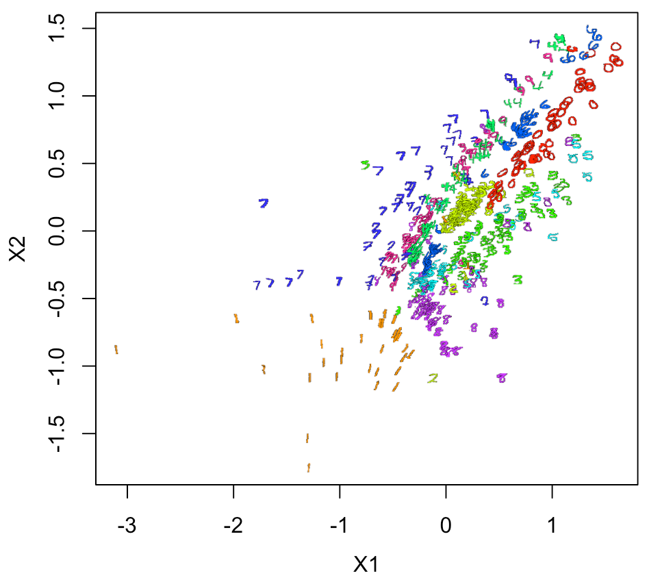
同じく、実際の画像での2Dプロットをやってみると

summary(Autoencoder3)
intermediate_layer <- keras_model(inputs = Autoencoder3$input,
                                  outputs = get_layer(Autoencoder3, "dense_3")$output)
summary(intermediate_layer)
intermediate_output <- predict(intermediate_layer, x_train)

xy <- data.frame(ytrain, intermediate_output)
Sam <- sample(1:nrow(xy), 500, replace = F)
xy1 <- xy[Sam,]
xy1[,2:3] <- log10(xy1[,2:3])
xy2 <- xtrain[Sam,,]

par(mfrow=c(1,1), mai=c(0.75,0.75,0.2,0.2), mgp = c(2,1,0))
plot(xy1[,2:3], pch=21, cex=0.1, col="white")
a <- range(xy1[,2][is.finite(xy1[,2])])
b <- range(xy1[,3][is.finite(xy1[,3])])
a1 <- diff(a)*0.015
b1 <- diff(b)*0.015

for(n in 1:nrow(xy1)){
  #n <-4
  v <- col2rgb(rainbow(10)[xy1[n,1] + 1]) / 255
  img = channel(xy2[n,,], 'rgb')
  img[,,1] <- img[,,1]*v[1]
  img[,,2] <- img[,,2]*v[2]
  img[,,3] <- img[,,3]*v[3]
  ff <- t(as.raster(img))
  ff[ff == "#000000"] <- "#00000000"
  rasterImage(ff, xy1[n,2]-a1, xy1[n,3]-b1, 
              xy1[n,2]+a1, xy1[n,3]+b1)
}
legend("topleft", legend = c(0:9), cex=0.6, pch=NA, text.col = rainbow(10), bg = "black")

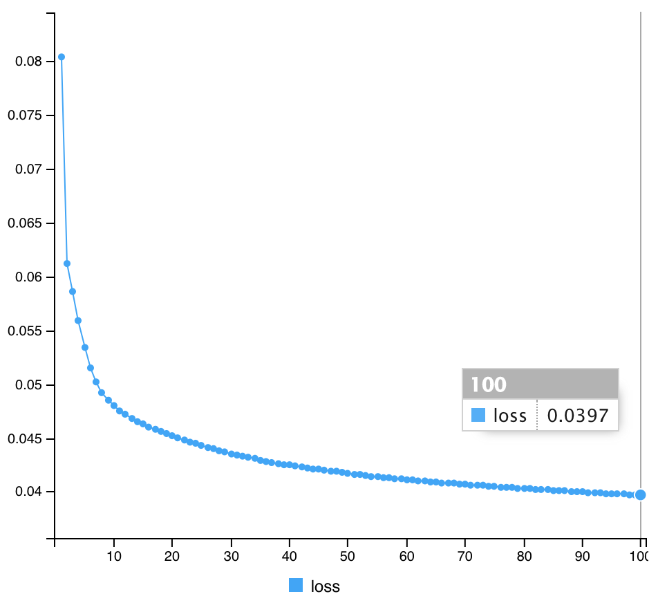
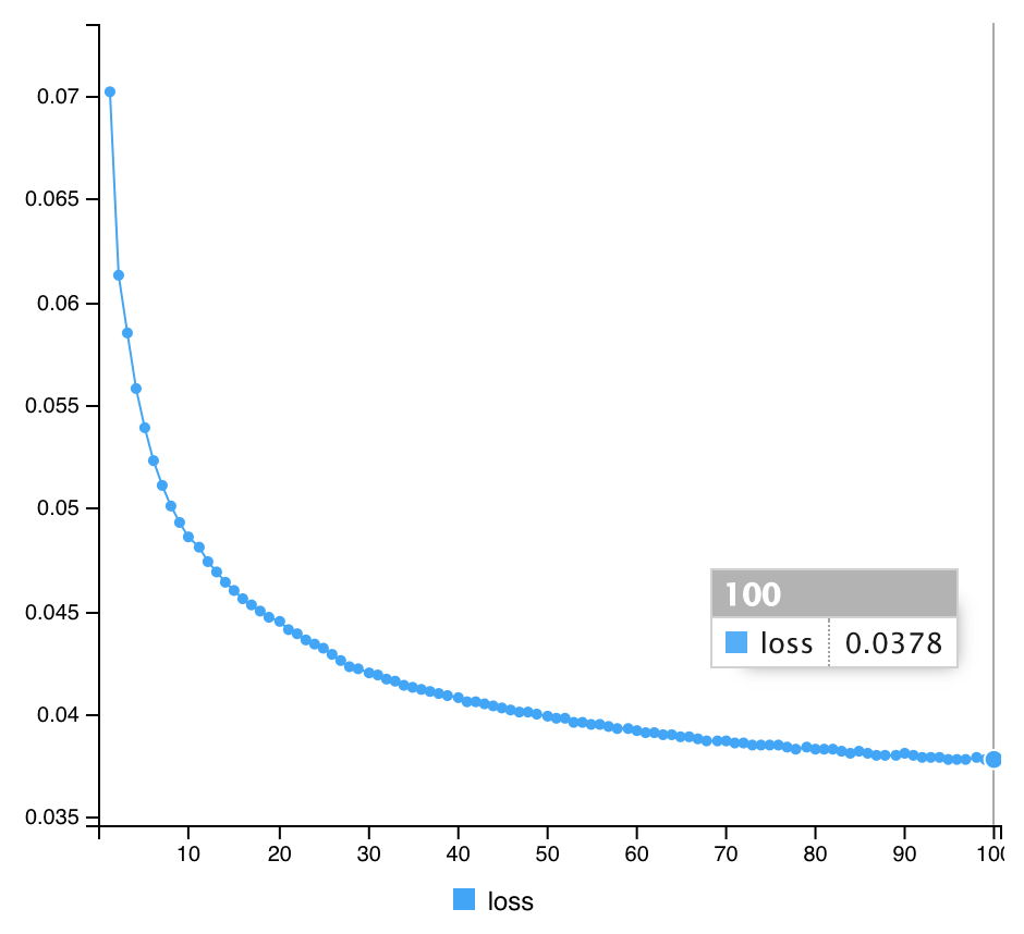
各モデルのlossの比較

Autoencoder	Final loss
Model 1	0.0397
Model 2	0.0378
Model 3	0.0358

結果、Science論文を参考にした、３番目のmodelが一番低くなった。

まとめ

いくつかのAutoencoder Modelを、R/Keras/Tensorflowで実装した。

実際、Deep Autoencoderの初期の研究が Scienceに掲載されているとは知らなかった。

いまでも十分使えるし、その派生したアーティテクチャも多数生み出されている。それだけインパクトがある研究なんだと思う。

R/Kerasを用いたDeep Learningの推薦図書

全コード in Gist

AuroEncoder_K01.R · GitHub

補足

Rstudioにおける、Rセッションのリスタート

.rs.restartR()

Weights全体を取得する場合

autoencoder2_weights <- Autoencoder2 %>% keras::get_weights()
str(autoencoder2_weights)

参考文献

www.datatechnotes.com

https://statslab.eighty20.co.za/posts/autoencoders_keras_r/

tf.keras.utils.plot_model | TensorFlow v2.0.0

Using colorized PNG pictograms in R base plotsryouready.wordpress.com

*1:David E. Rumelhart et al., Learning Internal Representations by Error Propagation, 318-362, 1987., URL: https://apps.dtic.mil/dtic/tr/fulltext/u2/a164453.pdf

*2:Pierre Baldi, Autoencoders, Unsupervised Learning, and Deep Architectures, JMLR: Workshop and Conference Proceedings 27:37–50, 2012., URL: http://proceedings.mlr.press/v27/baldi12a/baldi12a.pdf

*3:G E Hinton, R R Salakhutdinov, Reducing the Dimensionality of Data With Neural Networks, Science 28;313(5786):504-7, 2006., URL: https://science.sciencemag.org/content/313/5786/504

*4:https://www.cs.toronto.edu/~hinton/science.pdf

*5:https://science.sciencemag.org/content/sci/suppl/2006/08/04/313.5786.504.DC1/Hinton.SOM.pdf

*6:https://statslab.eighty20.co.za/posts/autoencoders_keras_r/

*7:https://andrie.github.io/deepviz/index.html

*8:https://bioconductor.org/packages/release/bioc/html/EBImage.html

2020-06-05

Mac Jupyterで、RとかPythonとかシェルとかのセットアップをするの巻

Mac Python R Terminalコマンド Jupyter Terminalコマンド - python Homebrew - python

はじめに
- まずは、ターミナルを立ち上げて、Macの実行環境確認
jupyterの設定
まとめ
補足
- jupyterのipynbファイルをhtml出力する
- CentOSでのjupyter設定（python3.6バージョン）

はじめに

Jupyter (ジュピター) は、対話型プログラミング用のブラウザ・インターフェイスと言えば良いのかな。PythonとかRとか、数十のプログラミング言語の動作環境として使えるのが魅力である。

大別して、Jupyter notebook と Jupyter lab という２種類のタイプがある。

個人的には、Jupyter lab のほうが若干見やすいというくらいの違いという印象である。

Jupyterのインストールと、いくつかの言語のセットアップ法についてメモしておく*1。

まずは、ターミナルを立ち上げて、Macの実行環境確認

$ brew config

HOMEBREW_VERSION: 2.3.0-37-g49324ad
ORIGIN: https://github.com/Homebrew/brew
HEAD: 49324ad17fab39f3312c568b5404cbf86b089d17
Last commit: 3 hours ago
Core tap ORIGIN: https://github.com/Homebrew/homebrew-core
Core tap HEAD: d043c3bc993728c0c2f05ebb13f8515640aeef26
Core tap last commit: 5 hours ago
HOMEBREW_PREFIX: /usr/local
HOMEBREW_DISPLAY: /private/tmp/com.apple.launchd.j3r06eCwYV/org.macosforge.xquartz:0
HOMEBREW_MAKE_JOBS: 8
CPU: octa-core 64-bit kabylake
Homebrew Ruby: 2.6.3 => /System/Library/Frameworks/Ruby.framework/Versions/2.6/usr/bin/ruby
Clang: 11.0 build 1103
Git: 2.26.2 => /usr/local/bin/git
Curl: 7.64.1 => /usr/bin/curl
Java: 12.0.2, 1.8.0_91
macOS: 10.15.5-x86_64
CLT: 1103.0.32.62
Xcode: N/A
XQuartz: 2.7.11 => /opt/X11

$ which python
/usr/local/bin/python

$ python -V
Python 3.7.7

$ which pip3
/usr/local/bin/pip3

$ pip -V
pip 20.0.2 from /usr/local/lib/python3.7/site-packages/pip (python 3.7)

実行環境としては、 Python3.7とかpip3とかのパスが通ってるのを前提とする。

jupyterの設定

jupyter notebook のインストール

$ pip3 install jupyter

# notebook サーバー起動
$ jupyter notebook

jupyter notebookをいったん閉じる。

jupyter lab のインストール

$ pip3 install jupyterlab

# lab サーバー起動
$ jupyter lab

Jupyter labの起動画面はこんな感じ。

デフォルトだと、 http://localhost:8888/lab で繋がるはず。

アイコンはあるけど、このインストールだと python3のNotebookとConsoleしか起動できない。

いまさらながら、python2の設定（失敗）

$ brew install python2

Updating Homebrew...
==> Auto-updated Homebrew!
Updated 1 tap (homebrew/cask).
==> Updated Casks
carbon-copy-cloner                       goland

Error: No available formula with the name "python2" 
==> Searching for a previously deleted formula (in the last month)...
Error: No previously deleted formula found.
==> Searching for similarly named formulae...
Error: No similarly named formulae found.
==> Searching taps...
==> Searching taps on GitHub...
Error: No formulae found in taps.

残念ながら、"python2" のformulaは削除されたようだ。

Rの設定

RあるいはRStudioを起動

options(repos="https://cran.csiro.au")

install.packages(c('repr', 'IRdisplay', 'evaluate', 'crayon', 'pbdZMQ', 'devtools', 'uuid', 'digest'))

devtools::install_github('IRkernel/IRkernel', force = TRUE)

IRkernel::installspec(user = FALSE)

ここで、RあるいはRStudioを閉じて*2、Jupyter labを見てみると

Rのアイコンが増えている！！

ibashの設定

$ pip3 install bash_kernel

$ python -m bash_kernel.install

これで、Bashのアイコンをクリックすると、 Notebook/Consoleが起動する。

SPARQLの設定

$ pip3 install sparqlkernel

$ jupyter sparqlkernel install

ijsの設定

$ brew install pkg-config node zeromq

$ pip3 install --upgrade pyzmq jupyter

$ npm install -g ijavascript

$ ijsinstall

これを実行すると、以下のエラーが出力された。どうも、Xcodeのインストールが必要らしい。

もしijavascript が使いたいなら、Xcodeをインストールしましょう。

gyp: No Xcode or CLT version detected!
gyp ERR! configure error 
gyp ERR! stack Error: `gyp` failed with exit code: 1
gyp ERR! stack     at ChildProcess.onCpExit (/usr/local/lib/node_modules/npm/node_modules/node-gyp/lib/configure.js:351:16)
gyp ERR! stack     at ChildProcess.emit (events.js:315:20)
gyp ERR! stack     at Process.ChildProcess._handle.onexit (internal/child_process.js:276:12)
gyp ERR! System Darwin 19.5.0
gyp ERR! command "/usr/local/Cellar/node/14.4.0/bin/node" "/usr/local/lib/node_modules/npm/node_modules/node-gyp/bin/node-gyp.js" "rebuild"
gyp ERR! cwd /usr/local/lib/node_modules/ijavascript/node_modules/zeromq
gyp ERR! node -v v14.4.0
gyp ERR! node-gyp -v v5.1.0
gyp ERR! not ok 
npm ERR! code ELIFECYCLE
npm ERR! errno 1
npm ERR! zeromq@5.2.0 install: `node scripts/prebuild-install.js || (node scripts/preinstall.js && node-gyp rebuild)`
npm ERR! Exit status 1
npm ERR! 
npm ERR! Failed at the zeromq@5.2.0 install script.
npm ERR! This is probably not a problem with npm. There is likely additional logging output above.

npm ERR! A complete log of this run can be found in:
npm ERR!     /Users/skume/.npm/_logs/2020-06-04T18_41_57_773Z-debug.log

まとめ

最終的に、こういう感じのLauncherになった。

アイコンが簡単に増えても、言語処理能力が追いつかない。。。

補足

jupyterのipynbファイルをhtml出力する

$ pip3 install runipy

$ runipy src.ipynb out.ipynb

$ jupyter nbconvert out.ipynb --to html

CentOSでのjupyter設定（python3.6バージョン）

$ sudo yum install -y python36u python36u-libs python36u-devel python36u-pip

$ python3.6 -m pip install --upgrade pip

$ python3.6 -m pip install jupyter

*1:ただ、RStudioユーザーとしては特段使いやすさは感じてないんだけど。。。

*2:今回、エラーが出たが、IRkernelのインストールさえうまくいけば動くかも

はじめに

googletransライブラリのメリット・デメリット

googletransのインストール

reticulateのセットアップ

RからPython googletransを呼び出す

googletransの実行

まとめ

補足

Rから、Python ライブラリのヘルプ表示

googleLanguageRの「No authorization yet in this session!」問題を解決するのは面倒そう！【6/27追加】

参考資料

はじめに

Keras/TensorFlowのセットアップ

手書き文字MNISTデータセットの用意

Autoencoderのモデル構築

シンプルAutoencoderモデル ０１

RStudioセッションの初期化

シンプルAutoencoderモデル ０２

シンプルAutoencoderモデル ０３

各モデルのlossの比較

まとめ

R/Kerasを用いたDeep Learningの推薦図書

全コード in Gist

補足

参考文献

はじめに

まずは、 ターミナルを立ち上げて、Macの実行環境確認

jupyterの設定

jupyter notebook のインストール

jupyter lab のインストール

いまさらながら、python2の設定（失敗）

Rの設定

ibashの設定

SPARQLの設定

ijsの設定

まとめ

補足

jupyterのipynbファイルをhtml出力する

CentOSでのjupyter設定（python3.6バージョン）

`googletransライブラリ`のメリット・デメリット

`reticulate`のセットアップ

Rから`Python googletrans`を呼び出す

シンプルAutoencoderモデル０１

シンプルAutoencoderモデル０２

シンプルAutoencoderモデル０３

まずは、ターミナルを立ち上げて、Macの実行環境確認